The Pennsylvania State University, Spring 2021 Stat 415-001, Hyebin Song
Hypothesis Testing
Hypothesis TestingIntroduction to Hypothesis TestingLearning objectivesHypothesis testing frameworkHypothesisTest statistic and rejection regionTwo types of testing errorsTest statistic and p-valueSteps to perform a hypothesis testing with the significance level Duality of confidence intervals with hypothesis testsTests about one meanLearning objectiveSummaryTests about two meansLearning objectiveTwo independent samplesA paired sampleSummaryTests about proportions Learning objectiveOne sample (large n)One sample (exact)Two independent samples (large and )Test about variancesLearning objectiveTest about variancesMore examples on calculating Type I and II error probabilities and power of a statistical test Learning objectiveBest Rejection (=Critical) Regions and Likelihood Ratio TestsLearning objectivesComposite hypothesis and uniformly most powerful level test Simple null and composite alternative hypothesisLikelihood Ratio Tests (LRT)
Introduction to Hypothesis Testing
Learning objectives
- Understand the hypothesis testing framework
- Understand basic terminology in hypothesis testing framework
Hypothesis testing framework
Hypothesis
We have a parameter space , which can be partitioned into two nonoverlapping disjoint subsets and , i.e., .
is the set that is currently believed to contain the true parameter. The statistical problem of interest is to use the observed data to disprove the current (=null) hypothesis, .
- Null Hypothesis .
- Alternative Hypothesis (equivalently, ).
If there is sufficient evidence to disprove the null hypothesis from the observed data , we reject the null hypothesis (change of belief: ). Otherwise, we do not reject the null hypothesis (we do not make any changes in our current belief on ).
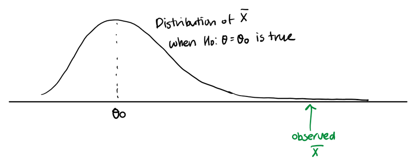
Sufficient evidence means it is unlikely to see the observed data if the null hypothesis is true. We need to decide how unlikely the data has to be to reject the null hypothesis.
Test statistic and rejection region
We use a test statistic and an associated rejection region (= critical region) to determine whether we have sufficient evidence to disprove the null hypothesis. We reject the null hypothesis if the observed test statistic is in the rejection region.
Remark : the decision is random, because the decision is based on the observed value of a test statistic. If we collect another sample, we would get a different observed test statistic value, and we may make a different decision.
Example: Let equal the breaking strength of a steel bar. Suppose follows a Normal distribution . If the bar is manufactured by process I, . The company recently changed the manufacturing process, and suspects that the breaking strength of a steel bar has increased while the variance of breaking strengths between steel bars remain the same. To test their hypothesis, the company sampled steel bars and recorded their breaking strengths. The sample mean of measurements was . The company claims that the breaking strength of a steel bar increased because the observed sample mean is greater than .
Hypothesis: .
A test statistic: .
An observed test statistic: .
A rejection region = .
Since is in the rejection region, the company rejected the null hypothesis.
Remark 1: In general, the form of rejection region is determined by the form of the alternative hypothesis . If
- , then the rejection region should be chosen as .
- , then the rejection region should be chosen as .
- , then the rejection region should be chosen as .
Remark: clearly, the large values of provides a stricter testing procedure. What value should we choose for ?
Two types of testing errors
For any fixed rejection region, two types of errors can be made in reaching a decision.
- Type 1 Error: reject when is true
- Type 2 Error: fail to reject when is true
The probability of a Type I error,
, is called the significance level of the test.
Example: What is the significance level of the test that the steel bar company bar in the previous example used? What would be the significance level of the test if the company decided to reject the null hypothesis if the observed test statistic is greater than ?
Test 1 (rejection region : )
P(rejecting when is true) =
Since
Test 2 (rejection region: )
P(rejecting when is true) =
Remark We usually fix the significance level of the test in advance (usually we let ), and make a decision rule so that the type 1 error of the test is .
Test statistic and p-value
So far, we have discussed how to determine whether we have sufficient evidence to reject the null hypothesis. The degree of sufficiency was determined by the significance level of the test.
- Given the significance level , if the observed test statistic falls into the rejection region associated with the significance level , we say, we have sufficient evidence to reject the null hypothesis at .
- Intuitively, if can reject the null hypothesis at a smaller value of , we have stronger evidence against the null hypothesis.
For example, in the steel bar example (),
- can reject the null hypothesis at , but not at .
- can reject the null hypothesis both and .
- can also reject the null hypothesis both and .
The p-value is defined as the smallest significance level of the test with which the null hypothesis can be rejected with the observed data.
For example, in the steel bar example (),
- the p-value when is the significance level of the test with the rejection region .
- the p-value when is the significance level of the test with the rejection region .
- the p-value when is the significance level of the test with the rejection region .
Therefore, p-value is the probability under the null hypothesis of obtaining a test statistic as extreme as the test statistic actually observed.
Remark 1: The smaller the p-value becomes, the more compelling is the evidence that the null hypothesis should be rejected.
Remark 2: the decision rule of "rejecting the null hypothesis when p-value is less than " is a level test.
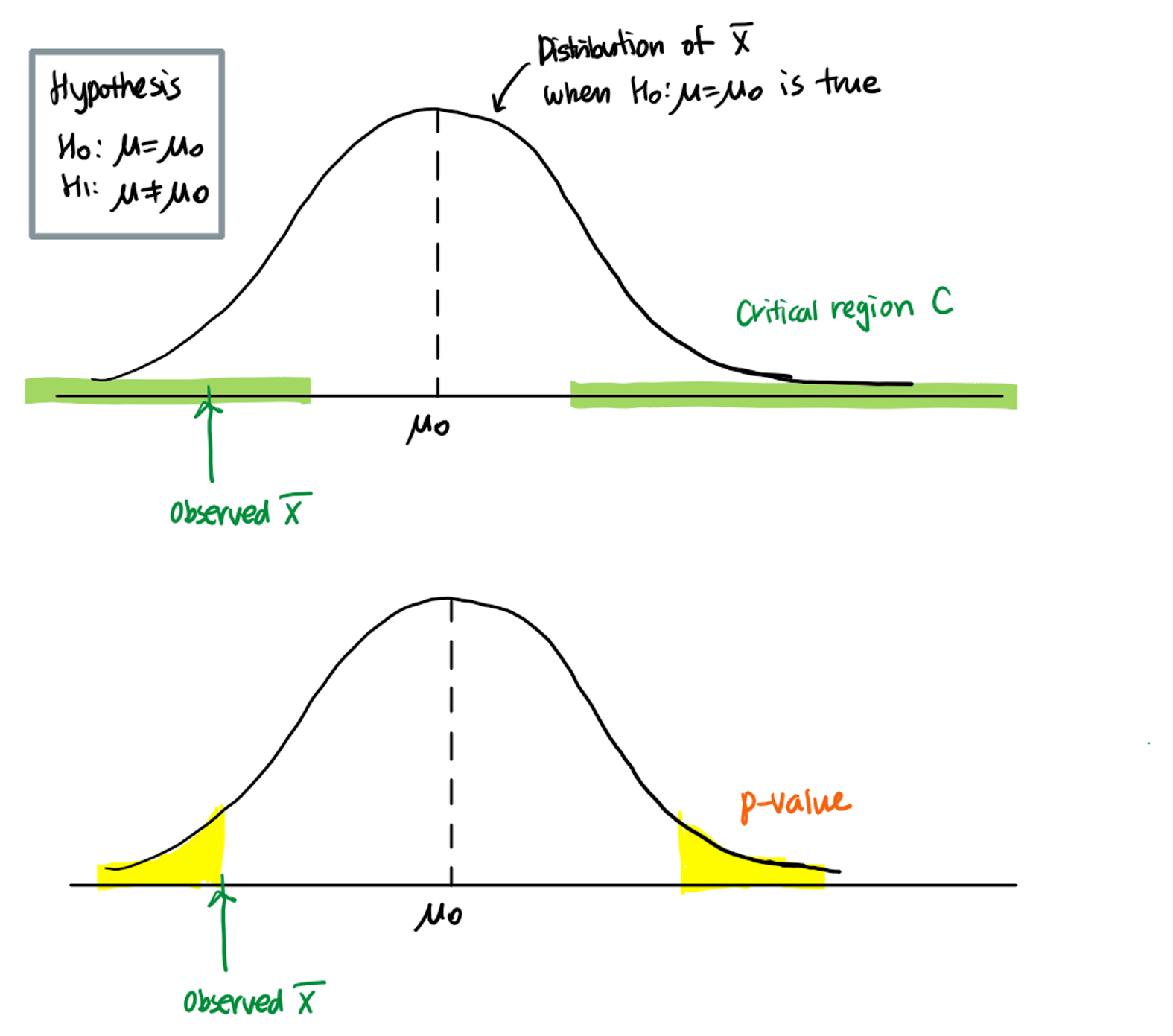
Example: Find the p-value when in the previous steel bar example (). Make a decision about the company's claim "the breaking strength of a steel bar has increased with the new manufacturing process" at the significance level of .
Rejection region:
p-value =
Do not reject the null hypothesis at .
Steps to perform a hypothesis testing with the significance level
- Write the null and alternative hypothesis.
null: ( is a fixed, known number)
alternative :
- one-sided: or
- two-sided:
Pick a a good estimator of . Choose a test statistic based on .
can be chosen as the test statistic.
Often, we work with a function of the estimator and whose distribution is free of . Usually, it is in the form of
- is often referred to as a standard error (SE) of an estimator
Find the distribution of the test statistic under the null hypothesis (i.e., when ).
Make a decision based on the observed value of the test statistic.
- Find a rejection region (=critical region) such that . Reject the null hypothesis if the observed test statistic is in the rejection region. or,
- Reject the null hypothesis if the p-value (associated with ) is less than .
Duality of confidence intervals with hypothesis tests
Recall that confidence intervals contain plausible values of the parameter of interest . Intuitively, we would think that if a confidence interval does not contain the hypothesized value , there is evidence against the null hypothesis .
There indeed exists an equivalence between hypothesis tests and confidence intervals. It can be shown that for the hypothesis and , the test statistic is outside of the rejection region associated with a significance level test if and only if the hypothesized value is not in the confidence interval. The decision rule is to
- reject the null hypothesis if the hypothesized value is not in the confidence interval. This decision rule is a significance level test.
Example: Construct a % confidence interval for , the breaking strength of a steel bar. The breaking strength of each steel bar follows a and the sample mean of steel bars was . Make a decision about the hypothesis that "the breaking strength of a steel bar is different from with the new manufacturing process" at the significance level of .
.
95% CI =
Since 50 is in the 95% CI, we do not reject the null hypothesis at .
The same duality principle holds for the one-sided hypotheses. For example, for the one-sided hypothesis
, we would reject the null hypothesis if the largest plausible value suggested by the data is still smaller than the hypothesized value . For this task, we need to construct a one-sided random interval with confidence coefficient such that . The corresponding confidence interval is . The decision rule is,
- for , reject the null hypothesis if .
- for , reject the null hypothesis if .
Recall that two-sided random intervals for are of the from
- A one-sided random interval with an upper bound :
- A one-sided random interval with a lower bound:
Example: Construct a one-sided % confidence interval which gives a lower bound for , the breaking strength of a steel bar. The breaking strength of each steel bar follows a and the sample mean of steel bars was . Make a decision about the company's claim "the breaking strength of a steel bar has increased from with the new manufacturing process" at the significance level of .
, .
A 95% CI with a lower bound =
Do not reject the null since
Tests about one mean
Learning objective
- Understand how to perform statistical hypothesis tests using three methods (rejection region, p-value, confidence interval) regarding the population mean
Setting
We have a random sample from some distribution. We would like to perform a hypothesis testing on the population mean of the distribution .
Null and alternative hypothesis:
or or
1. with known.
Hypothesis
- .
- .
- .
is a good estimator. Choose a test statistic :
Find the distribution of the test statistic .
- Under the null hypothesis , . Then , and therefore, .
Make a decision based on the observed value of the test statistic.
Method 1: choose a rejection region. We need to choose a rejection region so that
For three types of alternative hypotheses, we can choose rejection regions as
- :
- : .
- : .
Reject the null hypothesis if falls into the rejection region.
Method 2: compute the p-value.
- p-value when = significance level of the test with rejection region
- p-value when = significance level of the test with rejection region
- p-value when = significance level of the test with rejection region
Method 3: construct a confidence interval.
- : find confidence interval with an upper bound . Reject the null hypothesis if .
- : find confidence interval with a lower bound . Reject the null hypothesis if .
- : find confidence interval . Reject the null hypothesis if or .
Example: Let equal the length of life of a 60-watt light bulb marketed by a certain manufacturer. Assume that the distribution of is . Suppose the market standard life length of a 60-watt bulb is hours. The company wants to test whether the true length of life of a 60-watt light bulb is different from the market standard. A random sample of bulbs is tested until they burn out, yielding a sample mean of hours. Perform a statistical test on behalf of the company at the significance level .
- Hypothesis
- .
is a good estimator. Choose a test statistic
Find the distribution of the test statistic under the null hypothesis. Under the null hypothesis , . Then , and therefore, .
The observed test statistic is
- Rejection region: . Since , reject the null hypothesis at . OR,
- p-value = . Since p-value < , reject the null hypothesis at . OR,
- The confidence interval is . Since is not in the confidence interval, we reject the null hypothesis at .
2. with unknown.
Hypothesis
- .
- .
- .
is a good estimator. However, note is not a statistic anymore (because is unknown). We consider
Find the distribution of the test statistic .
Under the null hypothesis , . Then follows a distribution with degrees of freedom .
Lemma: i.i.d. Then, , i.e., a distribution with degrees of freedom of .
Make a decision based on the observed value of the test statistic.
Method 1: choose a rejection region. We need to choose a rejection region so that
For three types of alternative hypotheses, we can choose rejection regions as
- :
- : .
- : .
Reject the null hypothesis if falls into the rejection region.
Method 2: compute the p-value.
- p-value when = significance level of the test with rejection region
- p-value when = significance level of the test with rejection region
- p-value when = significance level of the test with rejection region
Method 3: construct a confidence interval.
- : find confidence interval with an upper bound . Reject the null hypothesis if .
- : find confidence interval with a lower bound . Reject the null hypothesis if .
- : find confidence interval . Reject the null hypothesis if or .
Example: In attempting to control the strength of the wastes discharged into a nearby river, a paper firm has taken a number of measures. Members of the firm believe that they have reduced the oxygen-consuming power of their wastes from a previous mean of . The observed values of the sample mean and sample standard deviation from sampled measurements were and . Suppose each measurement follows a Normal distribution. Perform a hypothesis testing for a significance level of .
- , .
- Test statistic:
- The distribution of under the null hypothesis is .
- The observed test statistic =
- Rejection Region:
- p-value: .
- 95% CI with an upper bound
3. from any distribution, large
Hypothesis
- .
- .
- .
is a good estimator. We consider
Find the distribution of the test statistic under the null.
By CLT, .
Since we have a large sample size,
Under the null hypothesis both test statistic follows a Normal distribution.
Make a decision based on the observed value of the test statistic.
Summary
When we have an i.i.d. random sample ,
| Settings | Test statistic |
|---|---|
| , known; . | |
| , unknown; . | |
| from any distribution, . | (approximate) or |
where is a sample variance estimator.
Tests about two means
Learning objective
- Understand how to perform statistical hypothesis tests using three methods (rejection region, p-value, confidence interval) regarding the difference of population means
Setting
We have two samples and from two groups, independent or paired. The goal is to test about the difference of population means of two groups, .
Null and alternative hypothesis:
or or
Two independent samples
1. Independent samples, , with known.
Hypothesis
- .
- .
- .
is a good estimator of . Choose a test statistic :
Find the distribution of the test statistic .
We have . Under the null hypothesis ,
, and therefore, .
Make a decision based on the observed value of the test statistic.
Given a significance level ,
- find a rejection region associated with the significance level
- find a p-value
- find a confidence interval of
Example: The amount of a certain trace element in blood is known to be normally distributed and vary with a standard deviation of 5 ppm (parts per million) for female donors and 10 ppm for male blood donors. Random samples of 25 female and 25 male donors yield concentration means of 33 and 28 ppm, respectively. A doctor wants to know whether the population means of concentrations of the element are higher for women.
- Hypothesis
- .
is a good estimator for . Choose a test statistic
Find the distribution of the test statistic under the null hypothesis. Under the null hypothesis .
The observed test statistic is
Rejection region: . Since , reject the null hypothesis at . OR,
p-value = . Since p-value < , reject the null hypothesis at . OR,
The one-sided confidence interval for is
Since is not in the one-sided confidence interval, we reject the null hypothesis at .
2. Independent samples, , with unknown variances
Hypothesis
- .
- .
- .
is a good estimator of . The test statistic in the previous setting,
is no longer a statistic anymore because are unknown.
1) unknown
We replace with a sample pooled variance estimator of , where . We consider the following test statistic
2) unknown, we use the following test statistic instead
Find the distribution of the test statistic .
1) unknown
- We have . Under the null hypothesis ,
2) unknown
We use Welch's approximation and obtain
- Make a decision based on the observed value of the test statistic.
Example: The amount of a certain trace element in human blood is known to be normally distributed. Also, it is known that the variances of this trace element are the same between men and women. Random samples of 25 female and 25 male donors yield concentration means of 33 and 28 ppm, respectively, with a standard deviation of 5 ppm for female donors and 10 ppm for male blood donors. A doctor wants to know whether the population means of concentrations of the element are higher for women.
- Hypothesis
- .
A test statistic
Find the distribution of the test statistic under the null hypothesis. Under the null hypothesis .
The observed test statistic is
- where . We have sample variance for women = and . Then, .
Rejection region: . Since , reject the null hypothesis at . OR,
p-value = . Since p-value < , reject the null hypothesis at . OR,
The one-sided confidence interval for is
Since is not in the one-sided confidence interval, we reject the null hypothesis at .
3. Independent samples, and , unknown distributions
Hypothesis
- .
- .
- .
is a good estimator of . Choose a test statistic :
when both variances are known or
when both variances are unknown.
Find the distribution of the test statistic .
From an application of a version of CLT, we have
and
since and when and are sufficiently large. Under the null hypothesis , .
- Make a decision based on the observed value of the test statistic.
A paired sample
When and are paired, we cannot use previous tests because and are dependent. Similarly as in the interval estimation, we consider another random variable , which is the difference between and . Note, . Therefore we can test
- <->
- <->
- <->
Assuming follows a normal distribution (or a large sample size), we can use the previous hypothesis testing procedure for one mean to test the hypotheses above.
Example A researcher wants to study whether lack of sleep impacts cognitive performance. The researcher recruited 10 participants. Each participant is asked to take the tests twice: one after a normal sleep and the other after being kept awake for 24 hours.
| 1 | 2 | 3 | 4 | 5 | 6 | 7 | 8 | 9 | 10 | |
|---|---|---|---|---|---|---|---|---|---|---|
| First test (normal sleep) | 8.1 | 9.5 | 7.2 | 11.6 | 9.9 | 7.3 | 10 | 10.7 | 10.4 | 8.5 |
| Second test (awake for 24 hours) | 7.0 | 8.6 | 6.3 | 10.7 | 8.8 | 6.3 | 8.9 | 9.1 | 9.0 | 7.5 |
Suppose it is reasonable to assume that the difference of test scores is normally distributed. The researcher wants to show that lack of sleep decreases cognitive performance.
- Hypothesis
- .
- A test statistic
- Find the distribution of the test statistic under the null hypothesis. Under the null hypothesis .
- The observed test statistic is
- p-value = . Since p-value < , reject the null hypothesis at .
Summary
When we have the observed sample , from two random samples ,
| Settings | Test statistic |
|---|---|
| , , independent, known; . | |
| , , independent unknown; . | |
| , , independent unknown; . | where is the df from Welch's approximation |
| Two independent random samples, large and ; . | (approximate) |
| Paired samples (dependent, ), when , unknown; . | |
| Paired samples (dependent, ), large ; | (approximate) |
where
- is a pooled sample variance estimator,
- is a sample variance estimator from ,
- is a sample variance estimator from ,
- is a sample variance estimator from where .
Tests about proportions
Learning objective
- Understand how to perform statistical hypothesis tests using three methods (rejection region, p-value, confidence interval) regarding the population proportion or difference of population proportions
One sample (large n)
Suppose we have a random sample . The goal is to test about the population proportion .
Null and alternative hypothesis:
- or or or .
is a good estimator of . Choose a test statistic :
By CLT, for , we have,
When ( is true), .
Make a decision based on the observed value of the test statistic . The decision rules which make an approximate level test are
RR: or or
p-value: or or
Remark: In step 2, we may consider,
Note under the null hypothesis, this test statistic also follows a standard normal distribution. Therefore, the test statistic can be used instead of in step 4. The test based on is called a score test, whereas the test based on is called a Wald test. There isn't any strong preference between two tests, although score tests tend to be preferred as they often result better approximations to a level significance tests.
Example: it was claimed that many commercially manufactured dice are not fair because "spots" are really indentations, so that, for example, the 6-side is lighter than the 1-side. Let equal the probability of rolling a six with one of these dice. To test against , several such dice will be rolled to yield a total of observations. Let equal the number of times that six resulted in the trials. The results of the experiment yielded .
- Make a conclusion based on the score test. Use
- Make a conclusion based on the Wald test. Use
Score test
- against
- Under the null, .
We reject the null hypothesis at since
Wald test
- against
- Under the null, .
We reject the null hypothesis at since
One sample (exact)
What if the sample size is too small to justify the use of CLT? In such case, we can no longer assume that the distribution of (score test statistic) or (Wald test statistic) under the null hypothesis is close to . The distribution of , where , is not equal to any common distribution that we usually work with. However, we know that the sum of i.i.d. Bernoulli random variables has a Binomial distribution.
Null and alternative hypothesis:
- or or or .
Choose a test statistic :
Since is sum of i.i.d. Bernoulli random variables where each , we have .
When ( is true), .
Make a decision based on the observed value of the test statistic .
RR:
- for such that .
- for such that .
- or such that .
p-value
or or
Example: Does pineapple belong on a pizza? people out of believe that pineapple belongs on a pizza. Test whether or not using the significance level %, where is the proportion of people who believe that pineapple belongs on a pizza.
and
Test statistic .
Under the null hypothesis, .
We have . Rejection region : or . We need to choose and such that , where .
k P(Y=k) 0 0.0156 1 0.0938 2 0.2344 3 0.3125 4 0.2344 5 0.0938 6 0.0156 Choose , . Then
Thus choose the rejection region or .
Since is not in the rejection region, we do not reject the null hypothesis at %.
P-value:
Since p-value is greater than , we do not reject the null hypothesis at %.
We have insufficient evidence to prove that the true proportion of people who believe that pineapple belongs on a pizza is different from %.
Two independent samples (large and )
Suppose we have independent samples, , . The goal is to test about the difference of population proportion .
Hypothesis
- .
- .
- .
is a good estimator of . Note under the null , and . Since under the null, both , we shall estimate with .
By an application of CLT,
Under the null, and since is large. Therefore, .
- Make a decision based on the observed value of the test statistic of .
Remark 1: Similarly in one sample case, the test statistic
can be alternatively used (Wald test).
Test about variances
Learning objective
- Understand one sample and two sample variance tests
Test about variances
Suppose we have a random sample . The goal is to test about the population variance .
Null and alternative hypothesis:
- or or or .
is a good estimator of . We might initially consider the scaled difference . However, this measure does not follow any common distribution, and also since is not a mean or sum of i.i.d random variables, CLT cannot be applied.
Recall the definition . From HTZ Theorem 5.5-2, we have,
That is, .
We consider the test statistic
Under the null hypothesis .
Make a decision based on the observed value of the test statistic . The decision rules which make a level test are
Rejection Region:
- :
- :
- : or .
p-value:
- :
- :
- :
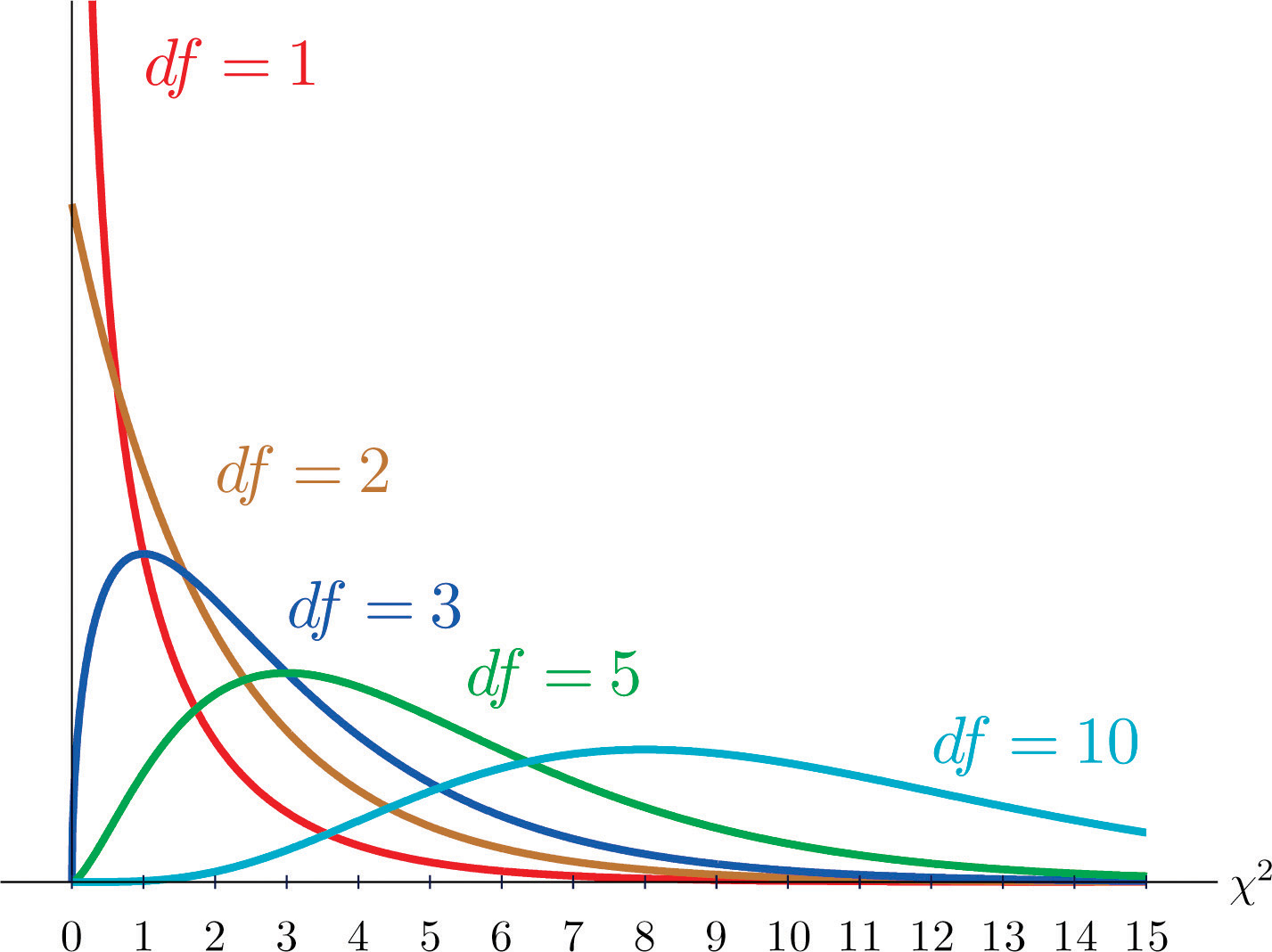
In R, can be obtained by
qchisq(p = 1-alpha,df = r)
Also, the probability that where can be computed in R via
xxxxxxxxxxpchisq(q = w, df = r)
Example: Consider a case in which pills are produced for treating a certain medical condition. It is critical that every pill have close to the recommended amount of the active ingredient because too little could render the pill ineffective and too much could be toxic. Suppose that a well-established manufacturing process produces pills for which the standard deviation of the amount of active ingredient is micrograms. Suppose further that a pharmaceutical company has developed a new process for producing the pills. The company wants to test whether the new process reduces the standard deviation of the amount of active ingredient from . A sample of size is taken, where the sample standard deviation of measurement was . Assume the amount of active ingredient in each pill follows a Normal distribution.
, .
Test statistic:
The distribution of under the null hypothesis is .
The observed test statistic is
Rejection region:
Since , we reject the null hypothesis.
or, p-value = where .
qchisq(p = 1-0.95,df = 22) # 12.338 pchisq(q = 10.78,df = 22) # 0.022
Now, suppose we have two independent random sample and The goal is to test about the difference of population variances and .
Null and alternative hypothesis:
- or or .
Remark: More generally, we can test or .
are good estimators of and . Similarly as in the one sample case, does not follow any common distribution, and also CLT cannot be applied.
We consider the test statistic
Fact: if and and are independent, then
the F distribution with degrees of freedom and .
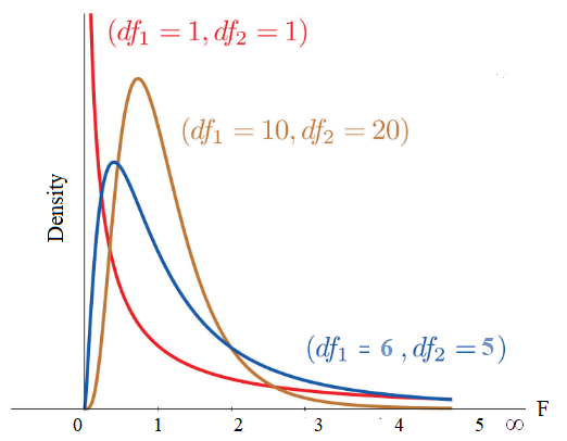
Recall, and . Thus,
Compute the observed test statistic .
The decision rules which make a level test are
Rejection Region:
- :
- :
- : or
Remark: it can be shown that . To see that, note is the number such that
where . Since where , independent, . Therefore,
Therefore, .
Thus, all cases can be written in terms of right-tail critical regions, and we have, rejection regions of
:
:
: or
Similarly, for p-values,
- : where
: where
- : where and .

Example A biologist who studies spiders believes that not only do female green lynx spiders tend to be longer than their male counterparts, but also the lengths of the female spiders seem to vary more than those of the male spiders. We shall test whether this latter belief is true. Suppose that the distribution of the length of male spiders is , the distribution of the length Y of female spiders is , and and are independent. We shall test against the alternative hypothesis . Suppose observations of yielded and while observations of yielded and . Use the significance level of 5%.
- and .
- Test statistic .
- The distribution of under the null is .
- The observed test statistic .
Rejection region is .
Since , reject the null hypothesis at = 5%.
qf(.05, 34, 26, lower.tail = F) = 1.879.
p-value = .
pf(3.205,34,26,lower.tail = F) = .0016
More examples on calculating Type I and II error probabilities and power of a statistical test
Learning objective
- Know how to compute type I and type II error probabilities for a given test and given a true parameter value
- Know how to find a power function of a given test
- Know how to find a required sample size to achieve certain statistical power
Recall for a statistical test, there are two types of errors
- Type I error: rejecting the null hypothesis when the null hypothesis is true.
- Type II error: not rejecting the null hypothesis when the alternative hypothesis is true.
Example
Assume that when given a name tag, a person puts it on either the right or left side. Let p equal the probability that the name tag is placed on the right side. We shall test the null hypothesis against the composite alternative hypothesis We shall give name tags to a random sample of people, denoting the placements of their name tags with Bernoulli random variables, , where if a person places the name tag on the right and if a person places the name tag on the left. Suppose people (out of 10) placed their name tags on the right. Since , for our test statistic, we use .
- Choose a rejection region so that the significance level of the test is less than or equal to %.
- Find the type II error probability when the true .
- Find the type II error probability when the true .
| p = 0.5 | p = 0.2 | p = 0.01 | |
|---|---|---|---|
| 0 | 0.0010 | 0.1074 | 0.9044 |
| 1 | 0.0098 | 0.2684 | 0.0914 |
| 2 | 0.0439 | 0.3020 | 0.0042 |
| 3 | 0.1172 | 0.2013 | 0.0001 |
| 4 | 0.2051 | 0.0881 | 0.0000 |
| 5 | 0.2461 | 0.0264 | 0.0000 |
| 6 | 0.2051 | 0.0055 | 0.0000 |
| 7 | 0.1172 | 0.0008 | 0.0000 |
| 8 | 0.0439 | 0.0001 | 0.0000 |
| 9 | 0.0098 | 0.0000 | 0.0000 |
| 10 | 0.0010 | 0.0000 | 0.0000 |
Solution
- and
- Test statistic
- Under the null hypothesis, ,
- Rejection region should be of the form . Choose such that the type I error probability under the null is less than %. In other words, .
Pmf of where .
Choose . . (Note, ). Due to the discrete nature of , it is not possible to construct a test such that the type I error probability is exactly 5%.
Rejection region: .
Type II error probability when = P(Not rejecting the null hypothesis when ) = .
Note when , the distribution of is .
Therefore,
Type II error probability when = P(Not rejecting the null hypothesis when ) = .
Definition: a power of the test at the parameter is defined to be the probability of rejecting the null hypothesis when the true parameter value is . In other words,
(If it is clear from the context which test is considered, is simply written as . In the book, is denoted as .)
Note, for , a power of the test at the parameter is 1-the type II error probability when , since
For example, in the name tag example above,
- power() = .
- power() = .
- power()= .
In fact, we can regard power as a function of the candidate parameter values.
.
Interactive plot for the power function
Example Consider the previous name tag example. Suppose a statistician wants to be silly, and consider a silly test: the statistician rejects the null hypothesis 5 % of the times regardless of the observed value of . Find the Type I error probability, and Type II error probability when . Find the power function of the test.
P(Type I error ; ) = 1/20.
P(Type II error ; ) = P(do not reject the null when ) = 19/20.
Power() = 1/20.
Note, this is a valid level test. However, the "power" of the test is terrible.
Remark 1: for a significance level test, the power curve is always below for by construction. We desire power() be as large as possible for (small risk of committing Type II errors.) Among all significance level tests, clearly, the best test to use is the one that results in the largest power for all (a.k.a., uniformly most powerful test).
Two questions: 1. does UMP test exist? 2. If so, how can we find the UMP test?
We will learn how to find a UMP test in some special cases. It is out of the scope of this class to provide more general answers to these questions. It is worth mentioning that most of the previously presented tests are optimal of some sort (they are either uniformly most powerful within level tests or uniformly most powerful within a more restricted class of tests if UMP does not exist within level tests).
Remark 2: Since we are already working with "optimal" tests, for a fixed sample size, both type I and type II error probabilities cannot be made arbitrarily small. For example, given a fixed sample size, we need to increase type I error probability to increase power. The only way of increasing power without increasing the type I error probability is to increase a sample size.
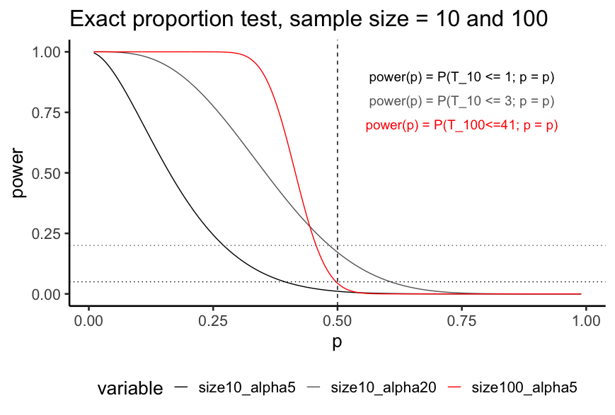
Remark 3: a fixed sample of size , the type II error probability depends on the distance between the true value and the hypothesized value . If is close to , the true value of (either or ) is difficult to detect, and the probability of accepting when is true tends to be large. On the other hand, if is far from , the true value is relatively easy to detect, and the type II error probability is considerably smaller.
Example Let be a random sample of size from the normal distribution , which we can suppose is a possible distribution of scores of students in a statistics course that uses a new method of teaching (e.g., computer-related materials).We wish to decide between (the no-change hypothesis because, let us say, this was the mean score by the previous method of teaching) and the researcher’s hypothesis Let us consider a sample of size and the test statistic .
- Choose the rejection region so that the test has the significance level of %.
- Find the type II error probability when .
- Find the power function of the test.
- What is the required sample size for the type II error probability to be less than % if the true parameter value is ?
and
Under the null (i.e., ), . Choose RR to be . Then .
When , Type II error probability = . Need to know the distribution of when .
Recall, . We have . When , .
Since ,
power() = P(Reject when ) = .
When , the distribution of = .
.
power() = .
When sample size is , . We want to find such that
We have the distribution of . Then the distribution of when is .
.
We need .
. i.e., .
Therefore is required.
Best Rejection (=Critical) Regions and Likelihood Ratio Tests
Learning objectives
- Know how to find a most powerful level test using Neyman-Pearson (NP) Lemma when both null and alternative hypotheses are simple.
- Know how to find a uniformly most powerful level test when the alternative hypothesis is composite and the best critical region from NP Lemma only depends on the null value.
- Know how to find a rejection region based on the likelihood ratio test.
Recall that a hypothesis is a statement about the location of the true parameter in the parameter space .
- E.g., where .
- In particular, for hypothesis tests, we constructed two hypotheses, and , where and
Definition [Simple and composite hypotheses] Suppose we have a random sample of size where each .
- A hypothesis is said to be a simple hypothesis if the hypothesis uniquely specifies the distribution of the population from which the sample is taken.
- Any hypothesis that is not a simple hypothesis is called a composite hypothesis.
Example 1 Suppose we have a random sample of size where each .
- :
- :
- :
- against :
Example 2 Suppose we have a random sample of size where each , unknown.
- :
Suppose that we would like to test a simple null hypothesis versus a simple alternative hypothesis . We would like to choose a test T so that
- the significance level of the test is , i.e., power.
- power is as large as possible
In other words, we seek a most powerful level test.
Remark: if two tests have different significance levels, they are not comparable.
The following theorem, Neyman-Pearson Lemma, provides the methodology for deriving the most powerful test for testing simple against simple . Before we present the theorem, let's consider the following example to build an intuition about the best rejection regions.
Example Suppose is a single observation from a normal population with unknown mean and known standard deviation . We want to test against .
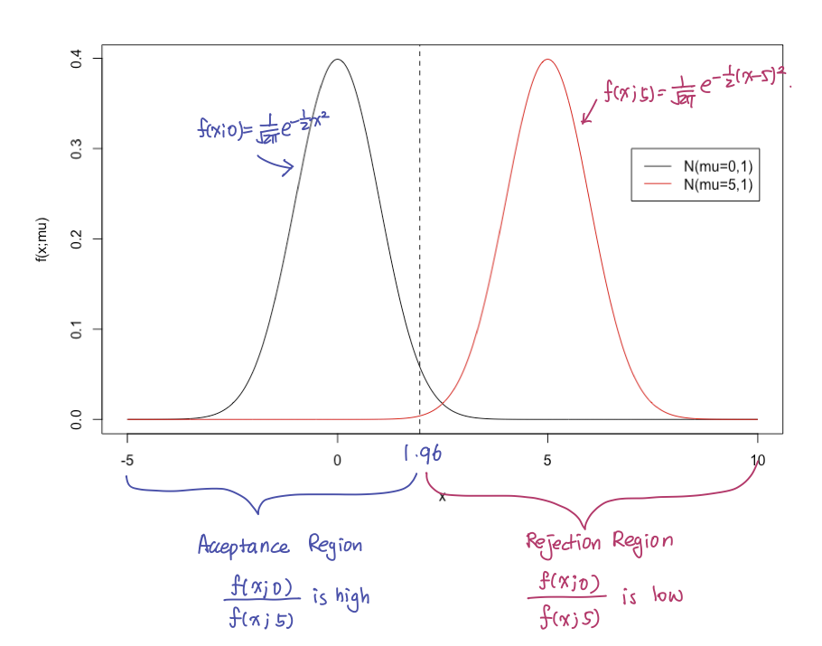
It makes sense to choose a rejection region where the ratio is small, because if the observed is in such region, it is likely to have come from (i.e., from the distribution with the pdf ).
Theorem [Neyman-Pearson Lemma]:
Suppose that we wish to test the simple null hypothesis vs. the simple alternative hypothesis . Let be a random sample of size with a distribution with pdf or pmf , where and are two possible values of . Let be the likelihood function, i.e.,
Then, for a given , the test that maximizes the power at has the rejection region, RR, determined by
The value of is chosen so that the test has the desired value for . Such a test is a most powerful level test for versus .
Remark: the rejection region based on NP Lemma can be equivalently defined via log-likelihoods.
Since is equivalent to , equivalently we can let the rejection region be
Example: Let be a random sample from . We shall find the best critical region of size for testing against .
By NP-Lemma, reject when the . (We shall choose later)
and therefore,
That is,
Equivalently,
,
i.e., for some .
So the problem (since depends on ) boils down to picking so that
.
Since when is true, .
Composite hypothesis and uniformly most powerful level test
Among the tests which have the same significance level , we prefer the test that has the largest power for all values of . Such test is called a uniformly most powerful level test.
Remark: Uniformly most powerful tests do not always exist. Especially, they usually do not exist when the composite alternative is two-sided ()
Simple null and composite alternative hypothesis
Suppose now we want to test against . If either hypothesis is composite, no general theorem comparable to NP-Lemma is applicable to find a level UMP test. However, the NP-Lemma can be applied to obtain a most powerful test for against , for any . If the same rejection region is obtained for any value of , the associated test should be a uniformly most powerful test.
In many situations, the actual rejection region for the most powerful test for vs. depends only on the value of (and does not depend on the value of ). In such case, a test obtained by the NP-Lemma is a uniformly most powerful test.
Example Let be a random sample from . We shall find the uniformly most powerful test of significance level for testing against .
Steps:
- Find the most powerful critical region for testing vs. , for each value of
- If the most powerful critical region is the same for each , then that critical region leads to a uniformly most powerful test of vs. the composite alternative
That is,
Equivalently,
,
i.e., for some ,
So the problem (since depends on ) again boils down to picking so that
.
Since when is true, .
Likelihood Ratio Tests (LRT)
The previous NP Lemma provides a method of constructing most powerful tests for simple hypotheses (i.e., under assumed hypotheses, the distribution of the observations is known).
Also, we have seen that NP Lemma can sometimes be used to find UMP tests for composite hypotheses that involve a single parameter (e.g. vs. where is an unknown parameter) by deriving a most powerful test for a simple alternative hypothesis (e.g. ) and checking that the rejection region of the test only depends on the assumed value in the null hypothesis ( in the example).
However, in many cases, the above strategy fails. For example, consider testing vs. based on a random sample when each and and are unknown.) Even though we consider vs. , both hypotheses are still composite, and we cannot use the previous rejection region based on the NP-Lemma.
We now present a very general method-Likelihood Ratio Test (LRT)-that can be used to derive tests of hypotheses.
Likelihood Ratio Test
Consider the following null and alternative hypotheses: and , where and are collections of possible values for such that .
Define by
Use as a test statistic. Reject if the test statistic is less than , where should be chosen based on the desired significance level of the test.
Remark 1: the previous method based on the NP-Lemma can be regarded as a special case of LRT.
Remark 2: for any .
Example: Suppose that is a random sample from a normal distribution with unknown mean and unknown variance . We want to test versus . Find the appropriate likelihood ratio test. Use .
As we can see from the previous example, an LR Test is often equivalent to a test based on a test statistic whose distribution under is known, and therefore such null distribution can be used to determine the rejection region of the LR test with significance level . Unfortunately, the likelihood ratio test does not always produce a test statistic with known null distribution.
Luckily, when the sample size is large, one can often carry out the likelihood ratio test directly in terms of using an asymptotic distribution of under the null hypothesis. Assume that the null parameter space is specified by restriction of the parameter space as
some coordinates of take fixed values.
For example, in the example above where , .
Under some mild regularity conditions, we have the following Theorem.
Theorem (asymptotic LRT; Wilks' Theorem) Let have joint likelihood function . Let denote the number of free parameters that are specified by and let denote the number of free parameters specified by the statement . Then, for large , has approximately a distribution with degrees of freedom. The test statistic, is called a LRT(Likelihood Ratio Test) Statistic.
The proof of this result uses a Taylor expansion and CLT and is beyond the scope of this class.
Example: consider the previous example (normal distribution with unknown mean and unknown variance ). We want to test versus . Suppose we have the sample mean of and sample standard deviation of from observations. Perform the exact and asymptotic likelihood ratio test at .
We have
LRT Test: reject if
Exact test
Choose such that .
From the above example, we know that
or for .
Since under , . We choose .
Exact LRT Test : reject if . Since , we fail to reject
Asymptotic LRT Test
Choose such that .
Since , choose such that .
Reject if .
Since ,
Since , we do not reject .